Federated Learning
Published:
Federated Learning is a way for server to train deep learning model without touching client data. It does so by outsourcing the training process to client node, and server only aggregates the model updates after such local training.
In the figure below, each client has a local model, which it trains locally using its private data. The device then upload the trained local model to a cloud server. The cloud server then calculate the update and let client download the update to continue training process.

In this notebook, I will make a demo to simulate Federated Learning process, including how client locally train a model, i.e. how the local model are generated, and how the cloud server gather the update and compute the global updated model, then send back to client.
In order to do so, let’s break down the components in this system:
- Server: Has a global model, has a way to send and receive models from client, has a function to aggregate the local update from client
- Client: Has a local dataset, has a way to train the model locally based on his dataset, has a way to send the update to server and receive the aggregated result from server.
Before we start, let’s review how a deep learning model look like. The model can be simplified as a stacked of multiple matrix multiplication: $y=W_n(…(W_1x+b_1)…)+b_n$. The “model” that we use to train is just a big list of matrices and vectors: $W_1,…,W_n$ and $b_1,…,b_n$. These matrices and vectors are not of the same shape, and in order to communicate $W$ and $b$ to central server, we would need to make them into a form of a long vector $v = \texttt{flat}(W_1,..,W_n,b_1,..,b_n)$. We would also need a function $\texttt{deflat}$ to convert back from $v$ to $W_1,..,W_n,b_1,..,b_n$.
In this notebook, we use two helper methods for that purpose in this notebook:
- A function to convert deep learning model to a vector for averaging at server
- A function to convert the vector back into the deep learning model to reconstruct the global update at client.
import torch

def model_to_vector(model):
  """
  Convert a PyTorch model to a vector of its weights.

  Args:
    model: A PyTorch model.

  Returns:
    A flattened vector of the model's weights.
  """
  vector = []
  for param in model.parameters():
    vector.append(param.data.view(-1))
  return torch.cat(vector)


def vector_to_model(vector, model):
  """
  Convert a vector of weights back to a PyTorch model.

  Args:
    vector: A flattened vector of weights.
    model: A PyTorch model (with the same architecture as the model used to create the vector).

  Returns:
    The PyTorch model with its weights updated from the vector.
  """
  offset = 0
  for param in model.parameters():
    param_size = param.data.numel()
    param.data = vector[offset:offset + param_size].view(param.data.shape)
    offset += param_size
  return model
# let's create some test code
from torchvision.models import resnet18

model = resnet18()
vector = model_to_vector(model)
print(vector.shape)
model_recon = vector_to_model(vector, model)
x = torch.rand(1, 3, 224, 224)
y = model_recon(x)
print(y.shape)
torch.Size([11689512])
torch.Size([1, 1000])
We see that the model input $x$ has a shape of $(1,3,244,244)$, which indicates an image of width 244, height 244, and 3 “channels”. These 3 channels are for coloring the image: R,G and B. A normal colored image has the value ranging from 0 to 255 at each pixel and each channel. We can try download an example image and print out the range of its value to see:
import matplotlib.pyplot as plt
plt.imshow(x[0].permute(1,2,0))
<matplotlib.image.AxesImage at 0x7b0f0b5ad0c0>
import matplotlib.pyplot as plt
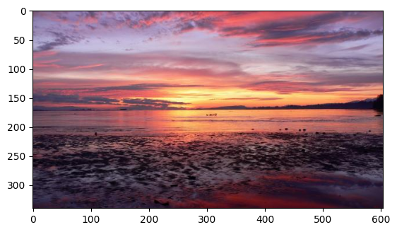
# download the image
!wget https://www.stockvault.net/data/2011/02/06/117454/thumb16.jpg -O test.jpg
img = plt.imread('test.jpg')
print(img.shape)
print("Image height: {}, Image width: {}, #channels: {}".format(img.shape[0],img.shape[1],img.shape[2]))
print("Range: {}-{}".format(img.min(), img.max()))
plt.imshow(img)
--2024-11-30 23:58:54--  https://www.stockvault.net/data/2011/02/06/117454/thumb16.jpg
Resolving www.stockvault.net (www.stockvault.net)... 104.26.11.44, 172.67.74.48, 104.26.10.44, ...
Connecting to www.stockvault.net (www.stockvault.net)|104.26.11.44|:443... connected.
HTTP request sent, awaiting response... 200 OK
Length: 35298 (34K) [image/jpeg]
Saving to: ‘test.jpg’

test.jpg            100%[===================>]  34.47K  --.-KB/s    in 0.004s

2024-11-30 23:58:54 (8.53 MB/s) - ‘test.jpg’ saved [35298/35298]

(340, 604, 3)
Image height: 340, Image width: 604, #channels: 3
Range: 0-255


<matplotlib.image.AxesImage at 0x7b0f0b621990>
In this demo, we will work on MNIST dataset, and have 10 clients, each hold a small dataset of 6000 digit images

Above is an example of MNIST images, it consists of 60000 images of digits, each image has size of 28x28
As the images are not colored, they only have 1 channel, making the whole shape of the input equals 784 = 28 x 28 x 1
# Let's start with a model
from torch import nn

class LogisiticRegression(nn.Module):
  def __init__(self, input_dim, output_dim, device = "cuda"):
    super(LogisiticRegression, self).__init__()
    self.linear = nn.Linear(input_dim, output_dim) # W,b Wx+b 784 -> 100
    self.device = device # GPU
    self.to(device)# pass the param to gpu

  def forward(self, x): #y = f(x)
    x = x.to(self.device) # pass the input to gpu
    x = nn.Flatten()(x) # make x into a 1d vector
    out = self.linear(x) # pass it through a linear layer, i.e. Wx+b

    return out # softmax will be applied later by loss function

def test_model():
  model = LogisiticRegression(784, 10) #784 = 28*28*1
  x = torch.randn(4, 28, 28)
  out = model(x)
  return out
  # print(out)


y = test_model()
print(y, y.shape)
tensor([[-0.1081,  0.2248, -0.4138, -0.5185,  0.0361,  0.7135, -0.0776, -0.0908,
         -0.1996,  1.5042],
        [-0.5581,  0.5065, -1.0035, -1.1533, -0.6793, -0.1168,  0.0972,  1.0448,
         -0.5441, -0.0458],
        [ 0.0676, -0.1420, -0.2188,  0.8619, -0.4488,  0.3295,  0.2454,  0.1947,
          0.6030,  0.3939],
        [ 1.2997,  0.7011,  0.3439,  0.6150,  0.6770,  0.7746,  0.4255,  0.0327,
         -1.3515,  0.9147]], device='cuda:0', grad_fn=<AddmmBackward0>) torch.Size([4, 10])
import torch
from torchvision import datasets, transforms
from torch.utils.data import random_split, DataLoader

# Load MNIST dataset
train_dataset = datasets.MNIST(root='./data', train=True, download=True, transform=transforms.ToTensor())

# Calculate the size of each partition
partition_size = len(train_dataset) // 10

# Split the dataset into 10 non-intersecting partitions
PARTITIONS = random_split(train_dataset, [partition_size] * 10 + [len(train_dataset) - partition_size * 10])[:-1]

# Print the size of each partition
for i, partition in enumerate(PARTITIONS):
  print(f"Partition {i+1}: {len(PARTITIONS[i])} samples")
Partition 1: 6000 samples
Partition 2: 6000 samples
Partition 3: 6000 samples
Partition 4: 6000 samples
Partition 5: 6000 samples
Partition 6: 6000 samples
Partition 7: 6000 samples
Partition 8: 6000 samples
Partition 9: 6000 samples
Partition 10: 6000 samples
Client class
Each client has a unique client id, and hold a set of local data of 6000 images, and a local model. It has a method to connect to the server, a method to receive update from the server, a method to locally train the model and a method to send the update to the server after training.
We also have “hyperparameters” for tuning the training at client: a local_batch_size for number of images being passed to the model at one training iteration, and a local_iteration number for how many iteration of training that we have at client side
from __future__ import annotations
# client class
class Client:
  def __init__(self, client_id, local_batch_size, local_iteration, device="cuda"):
    self.client_id = client_id
    self.local_bs = local_batch_size
    self.local_iter = local_iteration
    self.device = device
    self.data_loader = DataLoader(PARTITIONS[client_id], self.local_bs, shuffle = True)
    self.model = LogisiticRegression(784, 10, device)
    self.optimizer = torch.optim.SGD(self.model.parameters(), lr=0.1)
    self.loss_fn = nn.CrossEntropyLoss().to(device)
    self.losses = []

  def connect(self, server: Server):
    server.append_(self)

  # method to reconstruct the model from weight update
  def receive_update(self, update: torch.Tensor):
    self.model = vector_to_model(update, self.model)

  # method to locally train the data for local_iter round
  def local_train(self) -> None:
    iter = 0
    for batch_idx, (image, label) in enumerate(self.data_loader):
      self.optimizer.zero_grad()
      label = label.to(self.device)
      output = self.model(image).to(self.device)
      loss = self.loss_fn(output, label)
      loss.backward()
      self.optimizer.step()
      iter += 1
      if iter == self.local_iter:
        local_loss = loss.item()
        self.losses.append(local_loss)
        break

  def send_local_model(self)->torch.Tensor:
    return model_to_vector(self.model)
Server class
There is one central server. As mentioned above, the central server connect to a list of clients, and have a method to collect the updates from the client and make an aggregation. In this example, we simply do the update as average of all the local updates.
Server has one special parameters rounds, which indicates how many rounds do we want the training to last for. If we train for small number of rounds, the model quality may not be very good, while if we train for too long, it wastes the computing resource and the model might get overfitted.
from tqdm import tqdm
class Server:
  def __init__(self, rounds, device="cuda"):
    self.device = device
    self.model = LogisiticRegression(784, 10, device)
    self.clients = []
    self.rounds = rounds

  def append_(self, client: Client):
    self.clients.append(client)

  def train_round_(self):
    weights = []
    for client in self.clients:
      client.local_train()
      weights.append(client.send_local_model())
    new_update = self.aggregate(weights)
    for client in self.clients:
      client.receive_update(new_update)
    return new_update

  def aggregate(self, weights: torch.Tensor):
    return torch.mean(torch.stack(weights), dim=0)

  def train(self):
    for i in tqdm(range(self.rounds)):
      last_update= self.train_round_()
    self.model = vector_to_model(last_update, self.model)
server = Server(100)
for i in range(10):
  client = Client(client_id = i, local_batch_size = 32, local_iteration = 4)
  client.connect(server)
server.train()
100%|██████████| 100/100 [00:21<00:00, 4.76it/s]
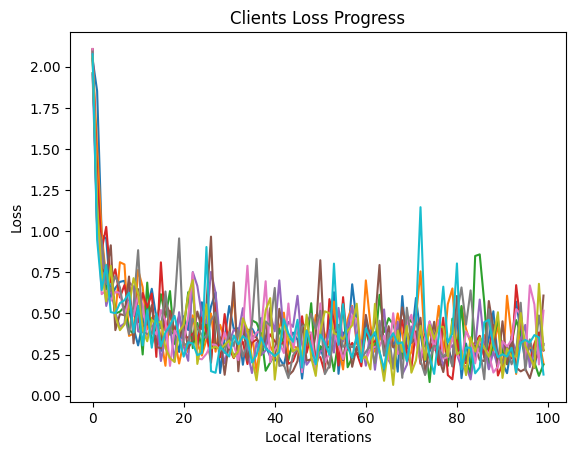
Let’s plot out the loss behavior. In Machine Learning, the loss indicates how “close” the predicted value and the targeted value is in the training dataset. So if the loss decreases over time, it is a good indication showing the training is successful.
import matplotlib.pyplot as plt
# plot clients loss progress
for client in server.clients:
  plt.plot(client.losses)
plt.title("Clients Loss Progress")
plt.xlabel("Local Iterations")
plt.ylabel("Loss")
plt.show()
Test model performance
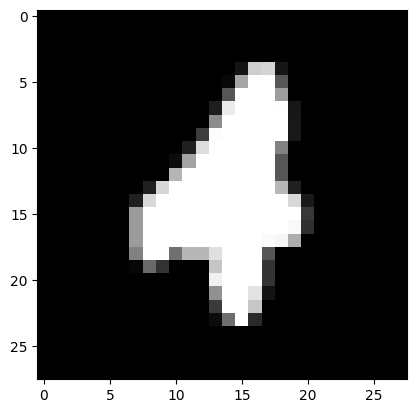
Now we first try to pick some sample and see if the model training is successful. We load the test dataset of MNIST, which the model has not been trained on. If the model can predict images on the test dataset, it shows the generalize performance of the model is good.
import random
# visualize an example
test_mnist = datasets.MNIST(root='./data', train=False, download=True, transform=transforms.ToTensor())
test_loader = torch.utils.data.DataLoader(dataset=test_mnist, batch_size=1, shuffle=False)
index = random.randint(0, len(test_mnist))
image, label = test_mnist[index]
prediction = server.model(image.to("cuda")).argmax().item()
print(f"Label: {label}, prediction: {prediction}")
plt.imshow(image.squeeze(), cmap='gray')
plt.show()
Label: 4, prediction: 4
Accuracy
Now we will compute how many percent of the test dataset does the model predict correctly with the accuracy function.
def accuracy(model):
  model.eval()
  correct = 0
  total = 0
  for images, labels in test_loader:
    output = model(images.to("cuda"))
    labels = labels.to("cuda")
    _, predicted = torch.max(output.data, 1)
    total += labels.size(0)
    correct += (predicted == labels).sum().item()
  return 100 * correct / total
acc = accuracy(server.model)
print("Final model testing accuracy: {}%".format(acc))
Final model testing accuracy: 91.59%
There are many ways we can make the model performance better/worse. We can change the set of parameters that mentioned above: local training iteration at client, batch size at client, the shared model between client and server, the total number of training rounds for Federated Learning.
–> Try to tweak all of the number and come up with a new model that can beat the performance we have at this notebook. <–
Leave a Comment